


Measurement setup and basics
Now the moment of truth strikes, once again. The test setup is finally final and the basis remains the well-known measurement microphone that has already proven itself for the in-ears. The suggestions for the realization I have found at Oratory and it does not hurt to look there once. But I think you should really measure the headsets and headphones properly and also underlay the usual hi-fi or gaming text wall with facts and not just list music tracks or games. Subjective perception and objective measurement in unison should be standard for reviews. The complete measurement setup and methodology is described in detail in the article linked below. We can save these redundant details. Nevertheless, it is recommended to have read this article at least once.
Important clue: The Harman curve
The so-called Harman Curve is an (optimal) sound signature that most people prefer in their headphones. It is thus an accurate representation of how, for example, high-quality speakers sound in an ideal room, and it shows the target frequency response of a perfect-sounding headphone. Thus it also explains which levels should be boosted and which should be attenuated based on this curve. This also explains in one fell swoop the term of the often quoted “bathtub tuning”, in which the Harman curve is, however, completely misused and exaggerated.
For this reason, the Harman curve (also called the “Harman target”) is one of the best frequency response standards for enjoying music with headphones, because compared to the flat frequency response (neutral curve), the bass and treble are slightly boosted in the Harman curve. This “curve” was created and published in 2012 by a team of scientists led by sound engineer Sean Olive. At the time, the research included extensive blind tests with different people testing different headphones. Based on what they then liked (or disliked), the researchers found and defined the most universally popular sound signature.
Matching headphones can be really problematic because of the human anatomy. Everyone has a slightly different pinna and ear canal, which affects how individuals perceive certain frequencies. In extreme cases, there is a few dB difference from person to person, which then explains the small differences in some measurements with artificial ears. Furthermore, if sound is not absorbed, it is additionally reflected by other surfaces. Theoretically, a torso could also be included in the test setup, but that would be much too time-consuming.
Measurement of the frequency response
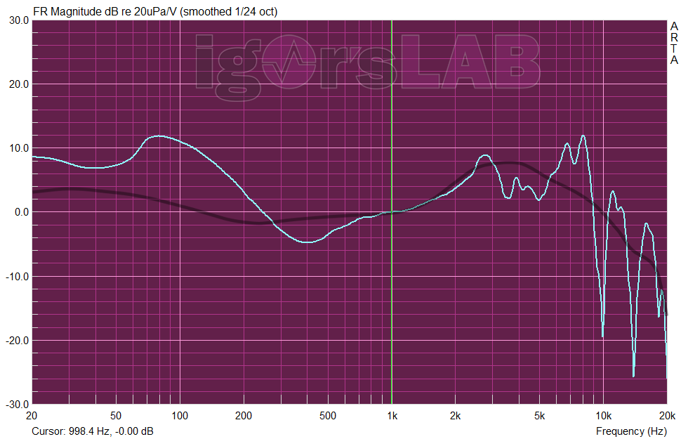
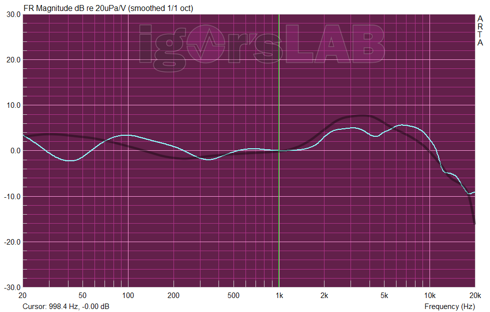
Let’s now move on to the measurement, where the Turtle Beach Stealth Pro was operated on the in-house wireless dongle (light turquoise curve). You can very nicely see an extreme curvature in the low frequency range up into the upper bass, which can be shifted significantly further to the right with different contact pressure. Then you have a disgustingly brutal upper bass that no one wants to have like that. So you have to be careful how you position the headset so that the measurement isn’t distorted. I have inserted the bad example grayed out for you, but in the following I refer to the measurements with the correct fit. Overall, the curve up to 1 KHz is extremely bass-heavy into the lower mids and with a deep hole in the mids. Then it goes steep again. The area around about 2.8 KHz shows a first peak followed by a slight dip at about 4.5 to 5 KHz.
The peaks at 7 to KHz stand for a slightly metallic sound, because it is really very sharp here. But more about that in a moment in the listening test. Above 10 KHz it gets lonely and the specification of 22 KHz as upper cutoff frequency is, because there is at least 8 dB difference to the 1 KHz mark. Yes, there is still something measurable, but usually tolerance ranges are given. The manufacturers of gaming headsets almost all leave these out. I certainly don’t have to explain why here. The 22 KHz is also pure marketing, because you don’t have bat ears anyway.
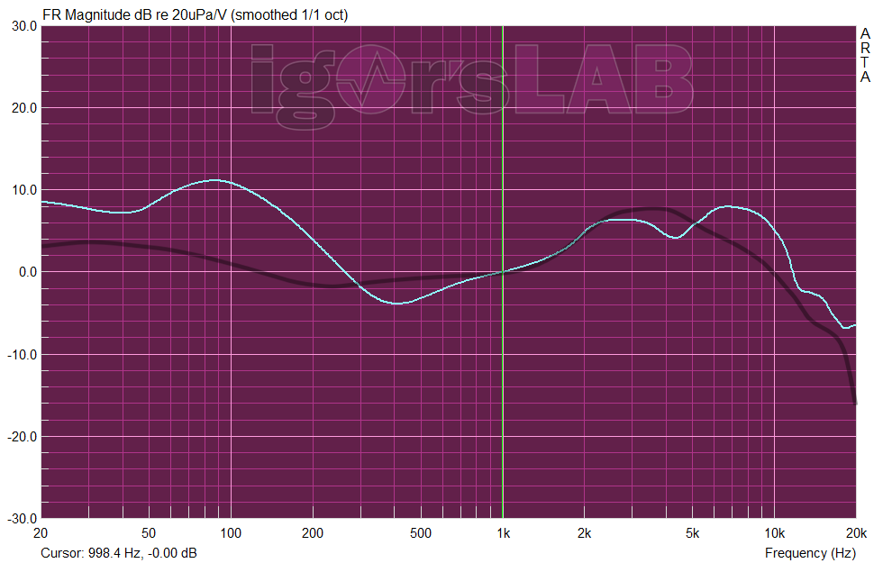
If we now smooth the whole thing down to the stop, we get a somewhat rounder curve, which, however, mainly confirms the criticism of the bass and the super high frequencies. The range of the lower mids is also too lax, which unfortunately robs the sound of some fullness and warmth, while the high frequency range becomes a whip in the super high frequency. You can’t really put it any clearer: this is pure gamer bathtub feeling.
Correction of the frequency response
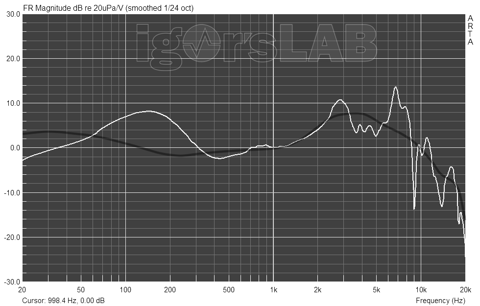
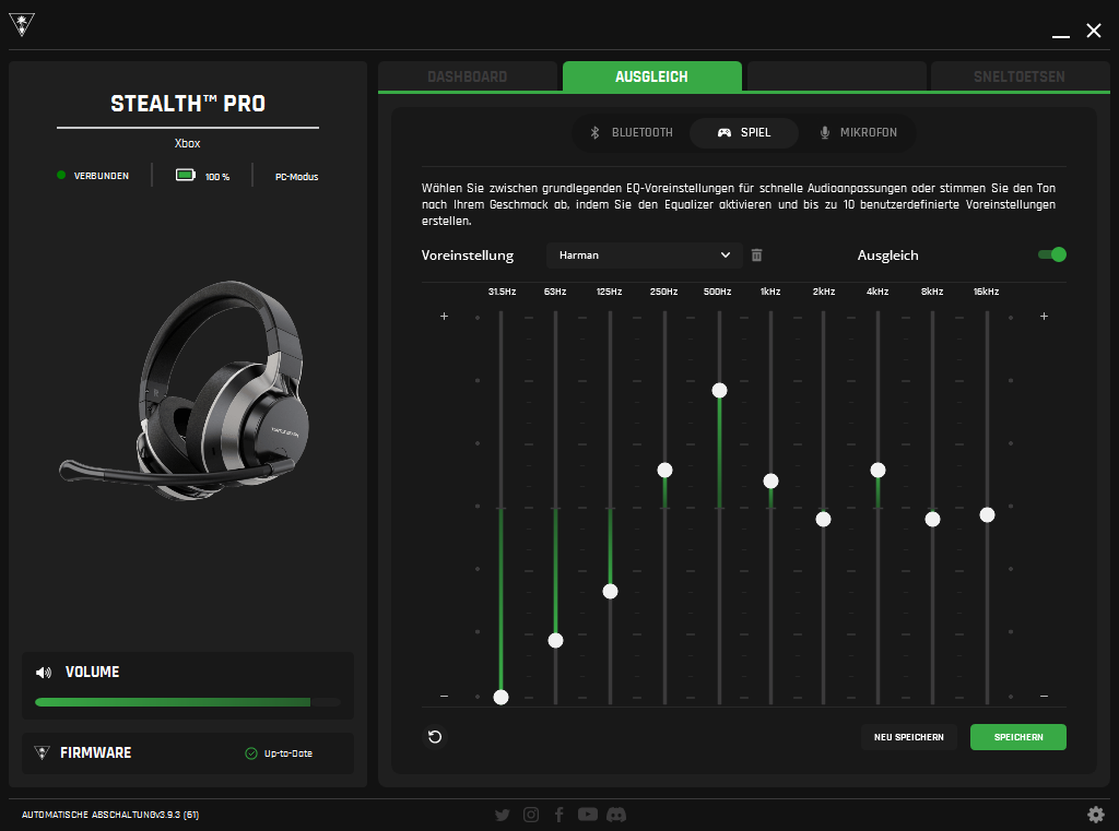
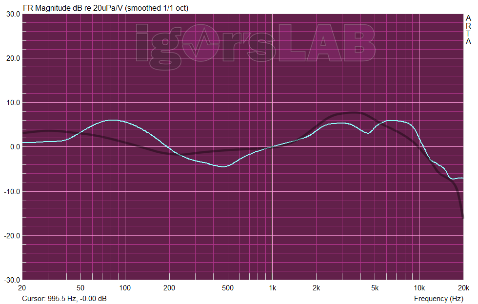
And now the app or softwares come into play, whereby the digital equalizer (EQ) is much too granular. Let’s first look at the result of the setting, which comes closest to the ideal curve. This looks quite useful, but the low bass also fails here due to the ear pads (dent at about 44 Hz), the rest looks and sounds quite good.
The software unfortunately reaches its limits here and if I MUST criticize something else: The sliders have no values and hitting the center position on a reset is nearly impossible. Even more stupid is that there is no real center reset, because what looks like it didn’t work for me. The only chance is to manually save the mean value (linear) as “Neutral Profile” before any change in all three tabs, and only then move the sliders. Sorry, but apart from the language confusion, this is rarely cumbersome and stupidly solved. I have created a Harman profile myself, which then looks like this:
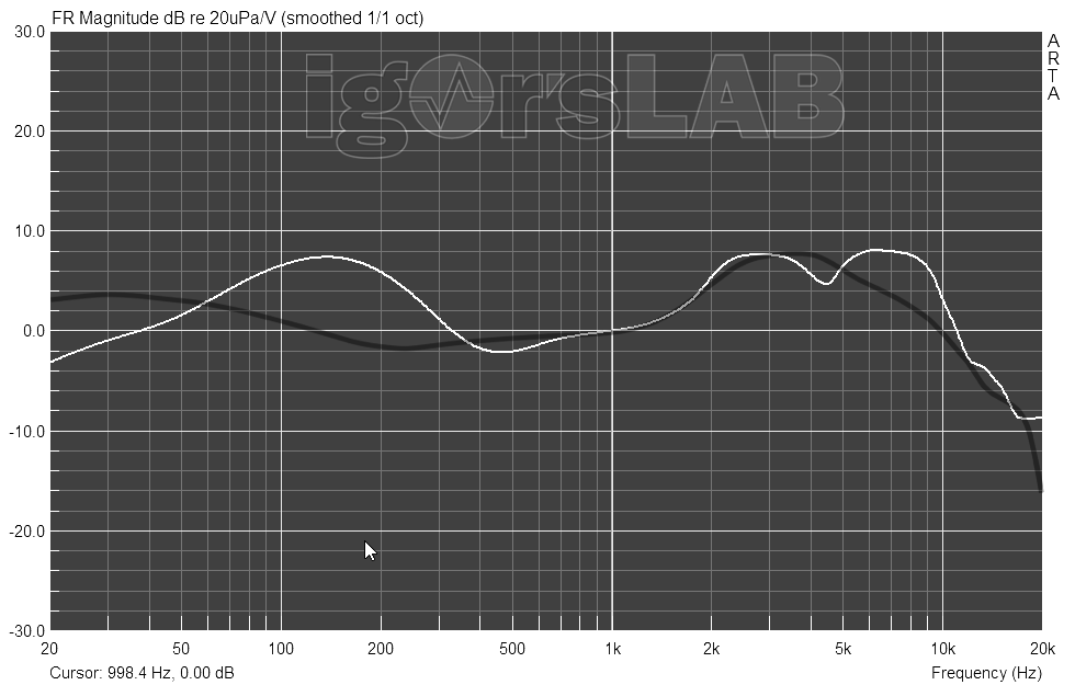
I also do not want to withhold the ANC and we can see the difference in the curve very clearly:
Cumulative spectra (CSD, SFT, Burst)
The cumulative spectrum refers to various types of plots showing time-frequency characteristics of the signal. They are generated by successively applying the Fourier transform and appropriate windows to overlapping signal blocks. These analyses are based on the frequency response diagram already shown above, but additionally contain the element of time and now show very clearly as a 3D graph (“waterfall”) how the frequency response evolves over time after the input signal has been stopped. Colloquially, this is also called “decay” or “decaying”. Normally, the driver should also stop as soon as possible after the input signal is gone. However, some frequencies (or even whole frequency ranges) will always decay slowly(er) and then continue to appear in this diagram as longer lasting frequencies on the time axis. From this you can easily see where the driver has glaring weaknesses, perhaps even particularly “clangs” or where in the worst case resonances could occur and disturb the overall picture.
Cumulative Spectral Decay (CSD)
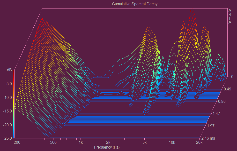
Cumulative spectral decay (CSD) uses the FFT and a modified rectangular window to analyze the spectral decay of the impulse response. It is mainly used to analyze the driver response. The CSD typically uses only a small FFT block shift (2-10 samples) to better visualize resonances throughout the frequency range, making it a useful tool for detecting resonances of the converter.
The picture shows very nicely the unsightly transient response and especially, the resonant response up to abundant 400 KHz. This is not a cleanly contoured bass, but a much too long lasting pad orgy without structure. Signal gone, sound gone? Not at all, because the bottom end resonates like a sack of doped bumblebees. You can also see the 2.8 kHz and 6 kHz metal whips very nicely, because there are still scratches on the eardrum when the signal has long since disappeared.
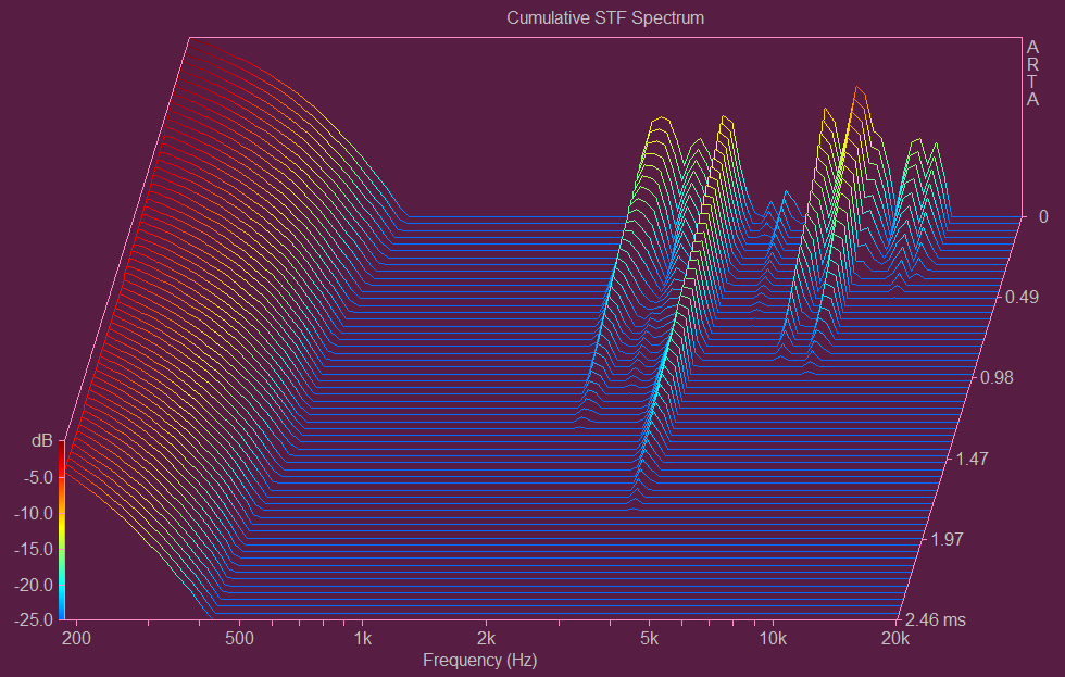
Short-time Fourier Transform (STF)
The Short-time Fourier Transform (STF) uses the FFT and Hanning window to analyze the time-varying spectrum of the recorded signals. Here, one generally uses a larger block shift (1/4 to 1/2 of the FFT length) to analyze a larger portion of the time-varying signal spectrum, especially approaching application areas such as speech and music. In the STF spectrum we can now also see very nicely the work of the drivers, which afford various weaknesses in some frequency ranges.
This “dragging” at the lower frequencies below 500 Hz is also clearly visible here, just like our acoustic domina with the bullwhips in the high frequencies. Too chunky at the bottom and partially too pointed at the top. In return, the area in between is almost completely anemic. Mids? No.
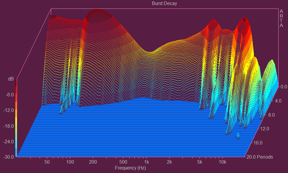
Burst Decay
With the CSD, the plot is generated in the time domain (ms), while the burst decay plot used here is represented in periods (cycles). And while both methods have their advantages and disadvantages (or limitations), it’s fair to say that plotting in periods may well be more useful for determining the decay of a driver with a wide bandwidth. And even there, the Turtle Beach Stealth Pro only performs quite mediocre. We mainly see strong resonance oscillations in the highs and the Kimos dent in the low bass.
The treble is probably supposed to sound particularly “crispy”, but it just grates on the nerves when you want to listen to music. For gaming, on the other hand, it is just okay, but the fun stops completely when listening to music (depending on the genre). The Turtle Beach Stealth Pro is relatively loud, but the overall level stability is only average.


37 Antworten
Kommentar
Lade neue Kommentare
Urgestein
1
Urgestein
Urgestein
Veteran
Urgestein
1
Urgestein
Urgestein
Urgestein
Urgestein
Urgestein
Urgestein
Urgestein
Urgestein
Urgestein
Urgestein
Urgestein
Veteran
Alle Kommentare lesen unter igor´sLAB Community →