OneOdio Monitor 80 Studio Headphones Review – Real Quality under 100 Euros, also for Gamers? Go!

1 - Introduction and technical data 2 - Optics, feel and wearing comfort 3 - Teardown: Pads, drivers and sounding 4 - Test setup, measurements and analyses 5 - Soundcheck, subjective sound analysis and conclusion

Measurement setup and basics

Now the moment of truth strikes, once again. The test setup is finally final and the basis remains the well-known measurement microphone that has already proven itself for the in-ears. The suggestions for the realization I have found at Oratory and it does not hurt to look there once. But I think you should really measure the headphones properly and also back up the usual hi-fi wall of text with facts and not just list music tracks. Subjective perception and objective measurement in unison should already be standard for reviews.

The complete measurement setup and methodology is described in detail in the article linked below. We can dispense with these redundant details. Nevertheless, it is recommended to have read this article at least once.

Final test setup for testing headphones and headsets – measuring instead of estimating and the backgrounds

Important clue: The Harman curve

The so-called Harman curve is an (optimal) sound signature that most people prefer in their headphones. It is thus an accurate representation of how, for example, high-quality loudspeakers sound in an ideal room, and it shows the target frequency response of perfectly sounding headphones. Thus, it also explains which levels should be boosted and which should be attenuated based on this curve. This also explains the term “bathtub tuning”, which is often cited, but in which the Harman curve is completely overused and exaggerated.

For this reason, the Harman curve (also called the “Harman target”) is one of the best frequency response standards for enjoying music with headphones, because compared to the flat frequency response (neutral curve), the bass and treble are slightly boosted in the Harman curve. This “curve” was created and published in 2012 by a team of scientists led by sound engineer Sean Olive. At the time, the research also included extensive blind tests with different people testing different headphones. Based on what they then liked (or disliked), the researchers found and defined the most universally popular sound signature.

Headphone tuning can be really problematic because of the human anatomy. Everyone has a slightly different pinna and ear canal, which affects how individuals perceive certain frequencies. In extreme cases, there is a few dB difference from person to person, which then explains the small differences in some measurements with artificial ears. Furthermore, if the sound is not absorbed, it is additionally reflected by other surfaces. Theoretically, a torso could also be included in the test setup, but that would be far too time-consuming.

Measurement of the frequency response

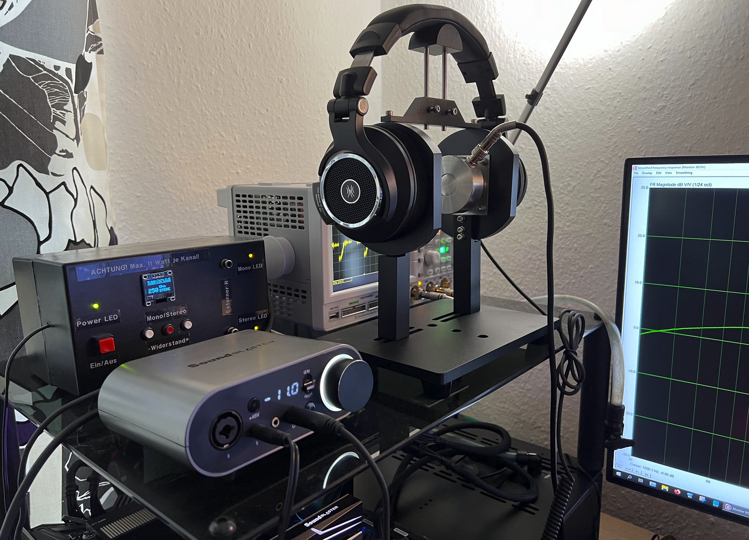
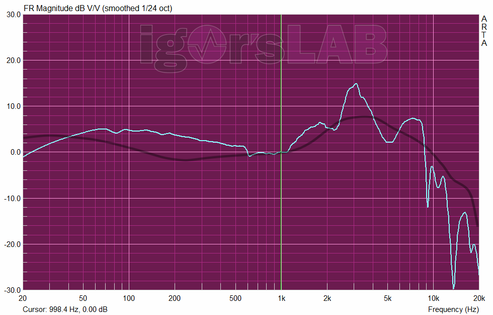
Let’s move on to the measurement, where the OneOdio Monitor 80 was operated in analog directly with the Creative Sound Blaster AE-9 as a reference (light turquoise curve). The output impedance of the AE-9’s power amplifier is well below one ohm, so that there are no impedance shifts and thus additional measurement errors, especially in the bass range. You can very nicely see a slight bulge in the low frequency range, which can be shifted even further to the left with more contact pressure. Overall, the response up to 1 KHz is very balanced and pleasant, but anything but completely neutral. The peaks at 3 KHz and 7 KHz are a bit too pronounced for my taste, while the super high frequencies start to run out of steam at around 10 KHz. Where a Hi-Res Audio logo is supposed to come from here, only the label buyer knows,

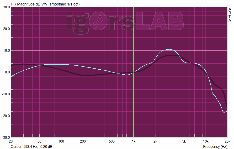
If you now smooth the whole thing down to the stop, you get a somewhat rounder curve, which, however, mainly confirms the point of criticism in the super high frequencies. The lower midrange is not over-present, but at least still gives the sound some fullness and warmth, while the bass remains pleasantly in the background without being completely absent. At 3 KHz, we again see the hearing-related level increase, which is slightly stronger than the ideal line of the Harman curve. In addition, the drivers overemphasize a bit in the super high frequencies at about 7 KHz, which drives the sibilants and blow-off noises of instruments into the metallic. It sounds a bit too crisp, but some people definitely like it. However, even after smoothing, we can see the slight deficits in the super high frequencies above about 10 KHz, where it goes down quite a bit.

Cumulative spectra (CSD, SFT, Burst)

The cumulative spectrum refers to various types of graphs showing time-frequency characteristics of the signal. They are generated by sequentially applying the Fourier transform and appropriate windows to overlapping signal blocks. These analyses are based on the frequency response diagram already shown above, but additionally contain the element of time and now show very clearly as a 3D graphic (“waterfall”) how the frequency response develops over time after the input signal has been stopped. Colloquially, such a thing is also called “fading out” or “swinging out”. Normally, the driver should also stop as soon as possible after the input signal is removed. However, some frequencies (or even whole frequency ranges) will always decay slowly(er) and then continue to appear in this diagram as longer lasting frequencies on the time axis. From this, you can easily see where the driver has glaring weaknesses, perhaps even particularly “clangs” or where resonances occur in the worst case and could disturb the overall picture.

Cumulative Spectral Decay (CSD)
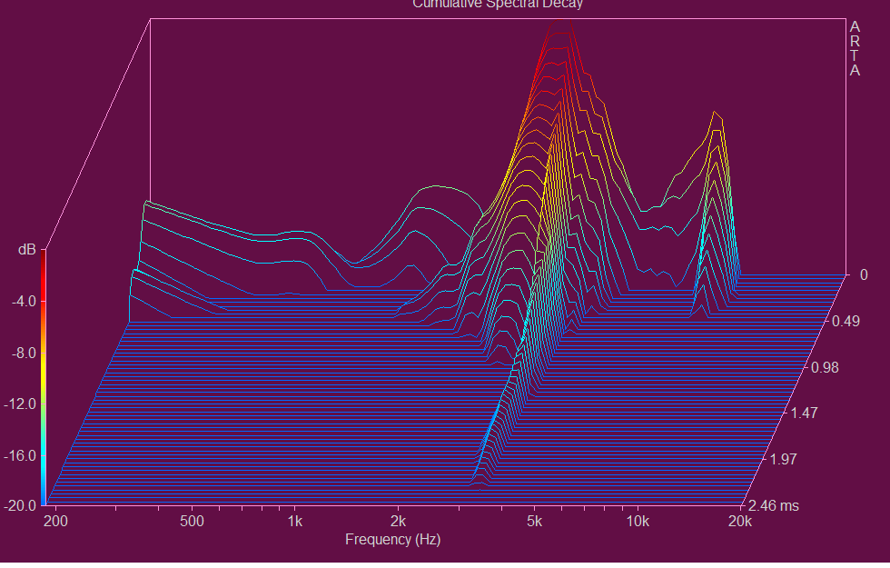
Cumulative spectral decay (CSD) uses the FFT and a modified rectangular window to analyze the spectral decay of the impulse response. It is mainly used to analyze the driver response. The CSD typically uses only a small FFT block shift (2-10 samples) to better visualize resonances throughout the frequency range, making it a useful tool for detecting resonances of the transducer.

The picture shows very nicely the transient response and the absolutely resonance-free course up to more than 1 KHz. For that alone, the just under 100 Euros would not be too much of a pity for me. You can analyze and dissect the individual sound layers very nicely and the fact that the peak only really dominates in a very narrow band at 3 KHz is also quite good. The cardboard sound in the lower mids is missing and only the slight overemphasis of the sibilants above 6 to 7 KHz brings us back down to earth.

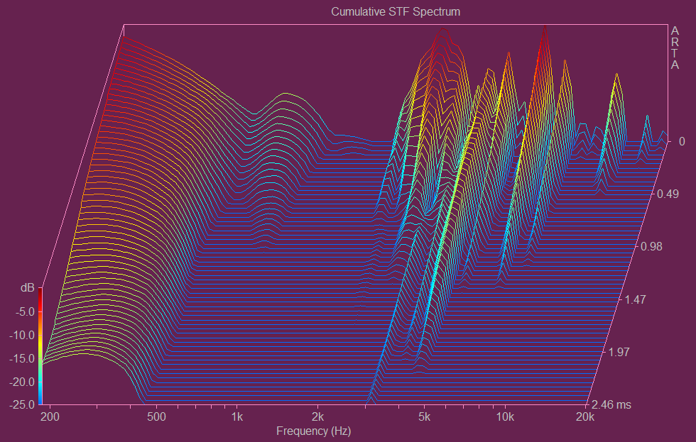
Short-time Fourier Transform (STF)
The Short-time Fourier Transform (STF) uses the FFT and Hanning window to analyze the time-varying spectrum of the recorded signals. Here, one generally uses a larger block shift (1/4 to 1/2 of the FFT length) to analyze a larger part of the time-varying signal spectrum, especially approaching application areas such as speech and music. In the STF spectrum we can now also see very nicely the work of the drivers, which afford various weaknesses in some frequency ranges.

This “dragging” at the lower frequencies below 500 Hz is then repeated several times between about 2.5 and about 10 kHz. I noticed in this context that, for example, very high bass frequencies at 40 to 70 Hz cause a kind of tremolo effect to set in in the mids above them, which “modulates” the mids. This is a bit unpleasant and you have to lower the level a bit, because the OneOdio Monitor 80 is not really level-proof.

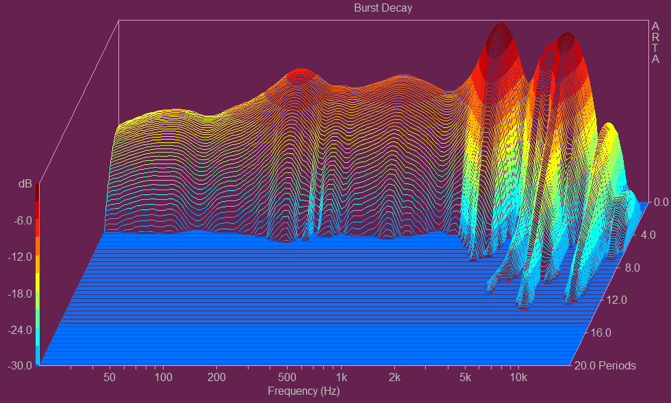
Burst Decay

In the CSD, the plot is generated in the time domain (ms), while the burst decay plot used here is represented in periods (cycles). And while both methods have their advantages and disadvantages (or limitations), it’s fair to say that plotting in periods may well be more useful for determining the decay of a driver with a wide bandwidth. And that’s exactly where the OneOdio Monitor 80 only performs mediocrely. We especially see strong resonance oscillations in the high frequencies again. This is probably supposed to sound especially “crispy”, but it also tugs at your nerves a bit when you want to listen to music. For gaming, on the other hand, it is okay (and almost seems intentional), but with music the fun more or less stops (depending on the genre).

Interim summary

The OneOdio Monitor 80 lacks level stability in the low bass, so it quickly pushes over the lower mids. However, this happens predominantly only with complex sound carpets. If you only have a few signal sources, this very level-dependent effect rarely occurs.